As turbine units grow and thermal systems become more complex and automated, flexible, reliable control is essential to safe, economic operation — demanding actuators with high torque, long stroke, high accuracy, multiple functions, fast tripping and fast modulation. Conventional valve actuators suffer sticking, lag and slowness, harming unit safety and economy. With the advance of mechano-electro-hydraulic integration, intelligent packaged electro-hydraulic actuators have been developed abroad: no external attachments, simple, reliable and easy to operate — the actuator of choice in some US plants in recent years.
An intelligent electro-hydraulic actuator integrates hydraulic, control, mechanical-electrical and computer technologies in two parts: the servo control system and the hydraulic drive system.
Fig. 1 shows the block diagram. It uses digital closed-loop control: position command and position feedback jointly drive a stepper motor, forming an ideal digital integrator; a measurement element detecting the moving parts directly closes the loop over all error sources and nonlinearities, and the computer controller applies deadbeat control. Positioning accuracy is thus set by the measurement element, disturbances and nonlinearities are dynamically corrected, and actual displacement tracks the command at all times with high dynamic accuracy.
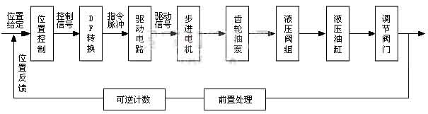
Fig. 1 Servo control system block diagram
The hydraulic circuit consists of a double-rod cylinder, valve group, bidirectional internal-gear pump, high-pressure solenoid valves and springs (Fig. 2). The bidirectional fixed-displacement internal-gear pump controls cylinder direction and speed by changing pump speed and flow direction; circuit pressure follows the load, so there is no surplus pressure or wasted flow — high efficiency. Return back-pressure acts directly on the pump inlet, becoming driving torque and reducing prime-mover power; hydraulic shock from reversing inertia is likewise recovered as pump-driving power. Direction changes via the pump produce little shock, suiting high-power, frequently reversing systems.
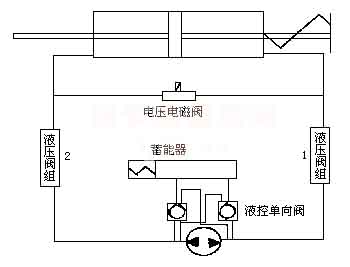
Fig. 2 Hydraulic drive circuit
Servo dynamics depend mainly on the position controller and the stepper motor. The stepper converts pulses into angular displacement: rotor angle and speed are proportional to pulse count and frequency, synchronised with the input pulses. Fig. 3 shows the dynamic structure of the closed-loop stepper position control system, comprising position controller, plant and feedback path.
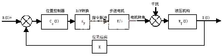
Fig. 3 Dynamic structure of the closed-loop stepper position control
From the position-control characteristics of the electro-hydraulic converter and deadbeat control theory, the generalised plant transfer function is:

Eq. (1) Generalised plant transfer function
Since the leakage coefficient can be reduced by manufacturing precision to the point of insignificance, it may be neglected and Eq. (1) becomes:
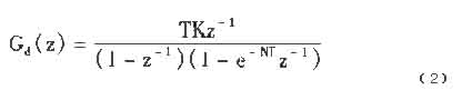
Eq. (2) Simplified transfer function
where T — position-sampling period; K — plant gain (K = K_F·K_θ·K_P·K_YA / V_C); N = (V_C + A²·E_Y)/V_C.
By the working principle of the internal-gear pump, its flow is:
Q = dv/dt = K_P · dΦ₁/dt (3)
Laplace-transforming Eq. (3), with pump flow as output and motor angle variation as input:
W(s) = Q(s)/Φ(s) = K_P·s (4)
From flow continuity, allowing for cylinder leakage and oil compressibility and noting that the hydraulic valve has no flow-regulating function, the circuit flow equation is:

Eq. (5) Circuit flow equation
Laplace-transforming Eq. (5), with flow as input and displacement as output:

Eq. (6) Circuit transfer function
From the analysis above and the system structure of Fig. 3, taking leakage coefficient K1 ≈ 0, the open-loop transfer function is:

Eq. (7) Open-loop transfer function
where Kd = K_F·K_θ·K_P·K is the system gain. With Kd = 280, the open-loop Bode plot from Eq. (7) is shown in Fig. 4.
By the Nyquist criterion — no open-loop poles in the right half-plane — the closed loop is stable if, below the gain crossover frequency ωc, the open-loop phase does not cross -180°, with phase margin γ of 30°–60° and gain margin of at least 4 dB.
From Fig. 4 the phase margin is 90° and the gain margin 11 dB, satisfying the Nyquist criterion — the system is stable.
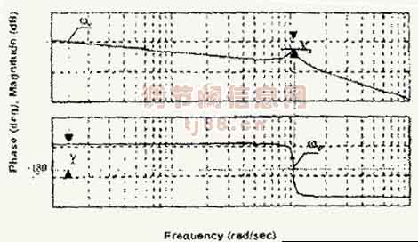
Fig. 4 Open-loop Bode plot of the control system
(1) The intelligent electro-hydraulic actuator system is stable and fast-responding; reducing gain, shortening cylinder stroke or adding damping all increase the stability margin. (2) Neglecting leakage, the system has no steady-state error — keeping leakage tiny improves dynamics and reduces error. (3) Direct valve regulation by the intelligent electro-hydraulic actuator saves capital and maintenance cost, and with its large force free of sticking and lag, raises safety and reliability substantially.